Get started with CraftGRN

CraftGRN is an R package for constructing and comparing condition-specific gene regulatory networks from matched ATAC-seq and RNA-seq data. The workflow follows three modules:

1. Predict TF binding sites from footprint or peak signal.
2. Connect TF binding sites to candidate target genes.
3. Learn regulatory topics and visualize differential GRNs.

The full pipeline is designed around a project YAML file that records paths, sample metadata, threshold values, genome settings, and output directories. For day-to-day analysis, the recommended workflow is wrapper-first: run one wrapper per module, then use the step functions when you want to inspect or customize a specific stage.

remotes::install_github("oncologylab/craftgrn")
library(craftgrn)

Demo data

CraftGRN keeps demo datasets outside the source package so installation remains small and CRAN-friendly. The package helper reports any configured external demo bundles:

craftgrn_demo_data_info()

No external demo bundle is currently configured. To run your own project, point CraftGRN at a project-level YAML file and use the normal Module 1 preparation function:

config <- "project.yaml"
module1_dir <- file.path(tempdir(), "predict_tf_binding_sites")

omics <- load_prep_multiomic_data(
  config = config,
  label_col = "strict_match_rna",
  do_preprocess = FALSE,
  verbose = TRUE
)

To run Module 1:

module1 <- predict_tfbs(
  omics_data = omics,
  out_dir = module1_dir,
  output_format = "auto",
  write_outputs = TRUE,
  write_stats = FALSE,
  verbose = TRUE
)

For project-level reproducibility, keep the run code in a short script beside the project YAML. The GSE192390 demo script follows this pattern: wrapper modes run full modules with one call, while step modes expose intermediate objects.

Sys.setenv(CRAFTGRN_DEMO_RUN_MODE = "full_wrapper")
source("11_pipeline_gse192390_tcell_fibroblast_demo.R")

Sys.setenv(CRAFTGRN_DEMO_RUN_MODE = "module3_steps")
source("11_pipeline_gse192390_tcell_fibroblast_demo.R")

Supported project-script modes should stay simple and explicit:

• module1_wrapper, module2_wrapper, and module3_wrapper run one module.
• module1_steps, module2_steps, and module3_steps expose intermediate objects for inspection.
• full_wrapper runs Modules 1, 2, and 3 through wrapper calls.
• full_steps runs Modules 1, 2, and 3 through step calls.

Troubleshooting demo data:

• If craftgrn_demo_data_info() returns zero rows, no public demo bundle is currently advertised by this package version.
• If file paths fail after moving the project, pass the project.yaml path explicitly. A portable config should use base_dir: "." so paths are relative to the config location.
• If the computer has limited memory, first run only load_prep_multiomic_data() and Module 1. Module 2 is larger because it computes TF-target correlations before restricting FP-target candidates to predicted TFBS.

Module 1: Predict TF binding sites

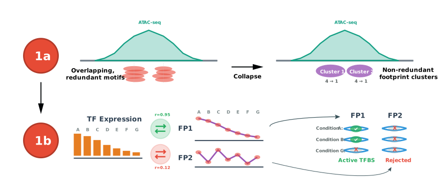
Module 1 combines normalized ATAC signal, RNA expression, footprint summaries, and sample metadata into a multiomic object. It aligns footprint sites, builds condition-specific binding flags, normalizes footprint scores, and predicts TF binding sites with a single user-facing workflow. Internally, CraftGRN first correlates each aligned footprint with the TFs represented by its canonical motifs, applies configured correlation cutoffs, and labels footprints with at least one canonical-bound TF. By default, only these canonical-bound footprints are used for the all-expressed-TF prediction step.

Inputs

Module 1 expects:

• A merged ATAC peak master table with normalized signal and overlap flags.
• A normalized RNA-seq count or expression matrix.
• A directory of per-condition motif footprint score and binding overview files generated by TOBIAS or a TOBIAS-compatible workflow.
• A metadata table mapping samples to conditions.
• A YAML configuration file with file paths, thresholds, and genome settings. The TFBS workflow uses threshold_fp_tf_corr_r, and can also use optional threshold_fp_tf_corr_p and threshold_fp_tf_corr_fdr fields when a project should require p-value or adjusted p-value support.

Supported built-in motif resources include hg38 and mm10.

For large projects, keep write_stats = FALSE and use output_format = "auto". Module 1 keeps full correlation tables as audit outputs, but the primary handoff to Module 2 is predicted_tfbs: a table with only aligned canonical-bound FPs and the TF names predicted to bind each FP.

Run Module 1

data_object <- load_prep_multiomic_data(
  config = "craftgrn_grn.yaml",
  genome = "hg38",
  gene_symbol_col = "HGNC"
)
module1_dir <- file.path(tempdir(), "predict_tf_binding_sites")

module1 <- predict_tfbs(
  data_object,
  out_dir = module1_dir,
  write_outputs = TRUE,
  output_format = "auto"
)

module1_qc <- build_module1_qc_report(
  module1,
  output_dir = file.path(module1_dir, "reports"),
  scan_predicted_tfbs = TRUE
)

Outputs

Module 1 creates:

• A CraftGRN multiomic object with normalized signal matrices, binary flags, and feature annotations.
• 01_fp_scores_qn_<db>.csv, the quantile-normalized footprint score matrix written for direct inspection and downstream external tools.
• Compact aligned footprint site, score, binding, and motif-support tables.
• Canonical-bound footprint summaries, including all canonical motifs retained for each aligned footprint.
• predicted_tfbs, the FP-to-TF handoff used by Module 2.
• Optional full TFBS correlation statistics for audit and debugging.
• module1_qc_report.html: an HTML QC report summarizing run parameters, input gates, motif-supported canonical support, correlation diagnostics, chunked predicted TFBS integrity, top TFs/FPs, condition support, motif complexity, warning checks, and related artifacts. The report uses static processing funnels, density curves, scatter summaries, heatmaps, lollipop rank plots, and cumulative curves.
• QC summaries reporting how many FPs, motif-supported pairs, canonical-bound FPs, prediction pairs, and predicted TFBS rows pass each step.

Module 2: Connect TFs to target genes

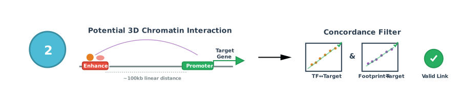
Module 2 treats TF-target prediction as a relational problem. It joins the Module 1 predicted_tfbs relation with TF-target expression correlations, restricted FP-target correlations, TSS-window evidence, and optional generic regulatory-prior evidence. GeneHancer, HiC, promoter-capture, CRISPR enhancer screens, or user tables are all represented as regulatory priors rather than separate modes.

Inputs

Module 2 uses:

• The CraftGRN multiomic object generated by Module 1.
• predicted_tfbs, with one row per predicted FP-TF binding event.
• A target gene TSS annotation table.
• Optional generic regulatory-prior FP-target links.
• YAML thresholds for TF-target and FP-target correlation filtering.

Process

Module 2 first computes TF expression to target expression correlations and filters TF-target pairs. Only after that filter does it build FP-target candidates from FPs bound by the surviving TFs. FP score to target expression correlations are computed only for those restricted FP-target candidates within the TSS window or supported by regulatory prior evidence.

module2 <- predict_tf_targets(
  multiomic_data = module1$omics_data,
  predicted_tfbs = module1$predicted_tfbs,
  gene_tss = gene_tss,
  regulatory_prior = regulatory_prior,
  project_config = "project.yaml",
  output_dir = file.path(tempdir(), "connect_tf_target_genes")
)

hnf4a_links <- query_predicted_links(module2, tf = "HNF4A")

module2_qc <- build_module2_qc_report(
  module2,
  multiomic_data = module1$omics_data,
  output_dir = file.path(tempdir(), "connect_tf_target_genes", "reports"),
  scan_large_tables = TRUE,
  validate_integrity = TRUE
)

Outputs

Module 2 produces normalized tables:

• module2_tf_target_corr: one row per TF-target correlation.
• module2_fp_target_candidates: one row per FP-target candidate with distance-to-TSS and prior evidence.
• module2_fp_target_corr: one row per FP-target correlation.
• module2_links: final TF-FP-target links as keys and pass flags.
• module2_condition_activity: long condition-level activity flags.
• module2_qc_summary: counts before and after each filter.
• module2_qc_report.html: a compact HTML review with sticky navigation and tabbed views for handoff checks, per-condition QC, TF-target and FP-target correlation filters, candidate source and distance-to-TSS evidence, final-link integrity, and top TF and target-gene summaries. Detailed values, warnings, output manifests, and related reports remain available in the technical appendix.

Module 3: Learn regulatory topics and visualize differential GRNs

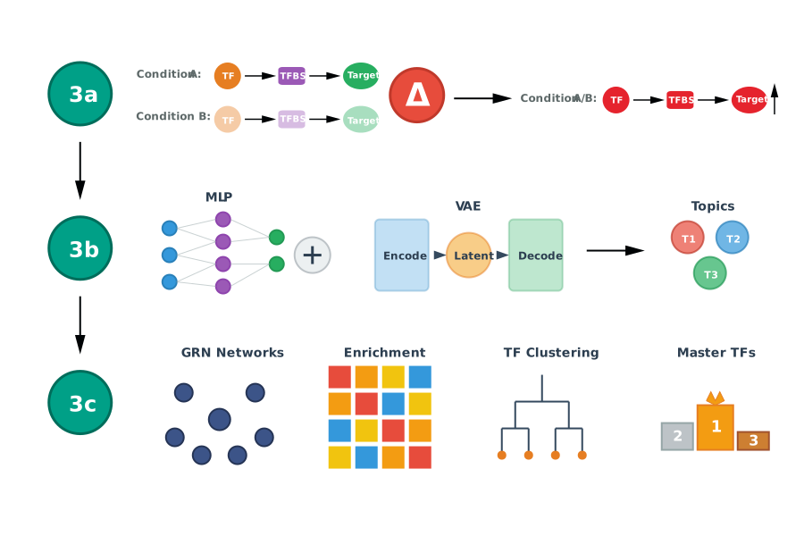
Module 3 compares regulatory links between conditions, builds joint RNA and footprint document-term matrices, trains topic models, assigns links to topics, and summarizes topic-specific pathway and master TF programs.

Inputs

Module 3 expects:

• Per-condition TF->TFBS->target link matrices from Module 2.
• A comparison metadata table defining pairwise contrasts.
• TF motif cluster assignments from Module 1.

Run regulatory topics

The topic modeling workflow builds documents such as comparison x TF-cluster x direction. Terms are genes and TFBS features, and weights are derived from RNA log2 fold changes and footprint or peak signal deltas. The model balances RNA and footprint contributions before converting weights into pseudocounts for topic modeling. By default, WarpLDA uses CraftGRN’s native warp_omp sampler, which keeps doc/word Metropolis-Hastings semantics while using OpenMP threads inside each model fit. For fixed-seed validation runs, set warplda_sampler = "warp_ref"; this native sequential reference sampler is much slower than warp_omp.

For regular analysis, keep one selected document construction method in the project YAML config. A standard run writes a flat single-method layout: topic_documents/, topic_models/, topic_extraction/, review/, and reports/. Benchmark-only method grids can be stored separately in the config and left disabled for normal package runs.

topic_method: comparison_aggr_multivi
topic_k: 10
warplda_iterations: 2000
topic_link_output: pass
topic_vae_device: auto
topic_vae_batch_size: 512
pathway_backend: enrichly
pathway_species: human_mouse_best

topic_benchmark_enabled: false
topic_benchmark_methods: []
topic_benchmark_k_grid: []

Use pathway_backend: enrichly for local cached pathway enrichment when the optional enrichly package is installed. Use pathway_backend: enrichr when you intentionally want the Enrichr web API backend. Use pathway_species: human, pathway_species: mouse, or pathway_species: human_mouse_best to choose pathway database behavior; if omitted, Module 3 infers the species from ref_genome when possible. The best-of mode runs human and mouse pathway databases separately and reports the better row for each topic and normalized pathway name, ranked by adjusted p-value, logp, combined score, and overlap size.

Pathway gene matching uses formal species-specific gene-symbol resolution when the relevant Bioconductor organism package is installed: org.Hs.eg.db for human and org.Mm.eg.db for mouse. CraftGRN resolves official symbols, case-insensitive symbols, aliases, ENSEMBL IDs, and ENTREZ IDs before comparing pathway inputs and returned overlap genes. If no formal match is available, it keeps a deterministic case-normalized fallback so old all-uppercase versus titlecase differences still match where possible.

Standard extraction folders are flat. For a selected K, review the K root for topic_terms.csv, topic_gene_peak_assignment.csv, topic_term_assignment_summary.csv, topic_links_pass.csv, topic_item_coverage_counts.csv, topic_terms_and_cutoffs_summary.pdf, topic_term_phi_score_heatmap_K*.pdf, topic_pathway_enrichment_dotplot.pdf, and per_comparison_topic_pathway_enrichment.csv. Standard runs do not create LDAvis, doc-topic heatmap, raw-theta document heatmap, topic pathway heatmap, standalone topic-term score heatmap, nested TF assignment, nested term assignment, or nested per-comparison pathway folders.

run_topic_modeling(
  filtered_dir = "differential_links",
  comparisons = "module3_comparisons.csv",
  output_dir = file.path(tempdir(), "regulatory_topics"),
  project_config = "project.yaml",
  run_training = TRUE,
  run_extraction = TRUE,
  run_reports = TRUE
)

The lower-level calls remain available when you want to inspect inputs, separate model training from topic extraction, or rerun only one stage.

module3_prepare_differential_links(
  module2 = "connect_tf_target_genes",
  multiomic_data = module3_multiomic,
  compar = "module3_comparisons.csv",
  project_config = "project.yaml",
  output_dir = file.path(tempdir(), "regulatory_topics", "differential_links")
)

module3_construct_docs(
  filtered_dir = file.path(tempdir(), "regulatory_topics", "differential_links"),
  output_dir = file.path(tempdir(), "regulatory_topics", "topic_documents"),
  tf_cluster_map = NULL,
  doc_mode = "tf",
  doc_design = "comparison",
  fp_term_mode = "aggregate",
  gene_term_mode = "unique",
  count_method = "log",
  include_tf_terms = TRUE
)

module3_train_topic_models(
  k_grid = 10,
  filtered_dir = file.path(tempdir(), "regulatory_topics", "differential_links"),
  output_dir = file.path(tempdir(), "regulatory_topics", "topic_models"),
  flat_output = TRUE,
  tf_cluster_map = NULL,
  doc_mode = "tf",
  doc_design = "comparison",
  fp_term_mode = "aggregate",
  gene_term_mode = "unique",
  count_method = "log",
  include_tf_terms = TRUE,
  backend = "vae",
  vae_variant = "multivi_encoder",
  vae_device = "auto"
)

module3_extract_topics(
  k = 10,
  model_dir = file.path(tempdir(), "regulatory_topics", "topic_models"),
  output_dir = file.path(tempdir(), "regulatory_topics", "topic_extraction"),
  topic_input_dir = file.path(tempdir(), "regulatory_topics", "topic_models"),
  backend = "vae",
  vae_variant = "multivi_encoder",
  doc_mode = "tf",
  weight_label = "peak_log2fc_fp_gene_fc_expr",
  flatten_single_output = TRUE,
  topic_report_args = list(link_topic_output = "pass")
)

Topic assignment interpretation

Module 3 uses different evidence for terms, TFs, genes, and links.

• Aggregate Gene and Peak terms are assigned from the topic-term matrix phi in two stages. The default topic_score_method = "normtop_specificity" downweights common non-specific terms before GammaFit identifies candidate topics. topic_term_assignment_method = "gammafit_maxprob" then requires the independently selected maximum-phi passing topics for matching GENE:<gene> and PEAK:<gene> terms to agree. Default GammaFit probabilities are model-specific.
• TFs are assigned from raw document-topic theta, not from topic links. A TF document such as comparison::TF::Target-Up belongs to a topic when theta >= topic_tf_membership_cutoff; the primary topic is the maximum-theta topic and ambiguity is controlled by topic_tf_primary_margin_cutoff.
• Genes are summarized from the topic terms observed in theta-selected documents. For per-comparison pathway analysis, a comparison/direction/topic gene set is the intersect of genes observed in documents with theta >= topic_tf_membership_cutoff and genes represented by the topic’s assigned GENE:<gene> and aggregate PEAK:<gene> terms.
• Physical TF-peak-gene links are not used to define pathway topic membership at extraction time. They can be projected later onto selected comparison/topic/pathway genes for subnetworks.

The standard coverage table topic_item_coverage_counts.csv reports Pass and Fail counts, fractions, and percentages for terms, genes, and TFs. TF coverage is document-theta based, so it does not change when only the topic-term GammaFit threshold changes.

When k_grid contains more than one value, the standard Module 3 output keeps the K-review tables and topic-model diagnostics for the selected method. Broad multi-method benchmarks are developer workflows and are not part of the normal package tutorial.

Review topic modeling and differential GRNs

build_module3_qc_report(
  topic_dir = file.path(tempdir(), "regulatory_topics"),
  differential_links_dir = "differential_links"
)

visualize_topic_modeling_results(
  topic_dir = file.path(tempdir(), "regulatory_topics"),
  output_dir = file.path(tempdir(), "regulatory_topics", "reports")
)

visualize_differential_grns(
  differential_links_dir = "differential_links",
  output_dir = file.path(tempdir(), "regulatory_topics", "reports"),
  top_tf_n = 10,
  top_link_n = 300
)

Outputs

Module 3 creates:

• Differential link tables, comparison-level plots, and an interactive differential GRN network browser with comparison, direction, Top TF, and Top link controls.
• Model selection metrics across topic-number choices.
• Topic-term and topic-link probability tables.
• Flat topic assignment tables, raw-theta document heatmaps, term-score heatmaps, overall pathway dotplots, and one per-comparison pathway retest table at the extraction root.
• Standard topic review tables and HTML reports under review/.
• Optional benchmark review tables and HTML reports under a separate benchmark output directory when topic_benchmark_enabled: true.
• module3_qc_report.html: a QC report summarizing topic inputs, method plan, theta separation scores, compact topic-link pass counts, and output files.
• Pathway enrichment summaries and plots.
• Master TF connectivity summaries and plots.
• Topic-stratified differential GRN visualizations.

Next steps

After running the three modules, inspect the model selection metrics, choose a topic number, review topic-specific pathway enrichments, and use master TF summaries to prioritize condition-specific regulatory programs for follow-up.